 Kashima's Office
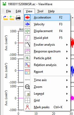
The [View] menu has submenus to select graphs and to change some visual settings on graphs. Most of submenus are titled graph types. By selecting a submenu, the specified graph is plotted as the current graph.
- Acceleration
- This submenu shows acceleration waveforms.
- Velocity
- This submenu shows velocity waveforms. The integration method to calculate the velocity can be selected from the Calculation] tab in the [Option] dialog box that can be opened from the menu [Tool] -> [Option].
- Displacement
- This submenu shows displacement waveforms. The integration method to calculate the displacement can be selected from the [Calculation] tab in the [Option] dialog box.
- Husid plot
- This submenu shows Husid plots. A Husid plot is the time history of the normalized Arias intensity.
- Fourier analysis
- This submenu contains the following sub-submenus. Those are results of the Fourier analysis.
- Fourier spectrum [amplitude]
- Power spectrum
- Auto correlation coefficient
- Response spectrum
- This submenu contains the following sub-submenus to select a type of response spectra.
- Acceleration response spectrum [Sa]
- Velocity response spectrum [Sv]
- Displacement response spectrum [Sd]
- Tripartite pseudo Sv [pSv]
- Energy spectrum [Ve]
The response spectrum is a plot of the maximum response of a single-degree-of-freedom system having a certain damping ratio as a function of its natural period. Three types of movement, i.e. acceleration, velocity and displacement, are treated as the response. So ViewWave acceleration [Sa], velocity [Sv] and displacement [Sd] response spectra.
Another response spectrum, which is called the pseudo response spectrum [pSv], is usually utilized in the tripartite plot of the response spectrum. The tripartite plot has horizontal and vertical axes scaled in logarithm and diagonal axes representing acceleration and displacement scales. If you specify a linear axis for the horizontal or vertical axis, the diagonal axes are not drawn. The pseudo response spectrum in ViewWave is calculated from the acceleration response spectrum.
The energy spectrum [Ve] is a plot of the total energy input to a single-degree-of-freedom system having a certain damping ratio as a function of its natural period.
- Particle orbit
- A type of the particle orbit can be selected from the following three sub-submenus.
- Acceleration
- Velocity
- Displacement
An acceleration sensor normally has three channels of data in the three directions orthogonal to each other. So the movement of a sensor is in three dimensions and can be projected to a plane. ViewWave calls such projection a particle orbit. This is also referred to as a Lissajous plot (or curve). As a particle orbit, ViewWave takes two channels being orthogonal and plots on an X-Y graph. Acceleration, velocity and displacement can be selected as the plotting data. A pair of channels for a particle orbit can be set in the [Channel] tab on the [Option] dialog box.
- Relation
- This submenu contains the following sub-submenus. Those are results of the relation analysis.
- Fourier spectral ratio [amplitude]
- Fourier spectral ratio [phase]
- Cross spectrum
- Cross-correlation coefficient
- Coherence
- Response spectral ratio
- Fourier spectral ratio [real]
- Fourier spectral ratio [imaginary]
Plural pairs of channels can be plotted in a graph and the combination of channels can be specified in the [Channel] tab on the [Option] dialog box.
- Report
- A report that is a combination of various graphs can be selected. Please refer to Setting - Report and Report for further information.
- Time axis
- Selecting one of the following sub-submenus, time axis of waveforms can be controlled.
- Backward: shifts waveforms backward.
- Forward: shifts waveforms forward.
- Magnify: magnifies time of waveforms.
- Reduce: reduces time of waveforms.
- Zoom
- Selecting one of the following sub-submenus, the graph is zoomed in or out.
- 50%: zooms out to 50% of original.
- 75%: zooms out to 75% of original.
- 100%: returns to original.
- 125%: zooms in to 125% of original.
- 150%: zooms in to 150% of original.
- 200%: zooms in to 200% of original.
- Legend
- Selecting one of the following sub-submenus, the legend position is changed.
- None: hides the legend.
- Upper left: places the legend on the upper left corner.
- Upper right: places the legend on the upper right corner.
- Lower left: places the legend on the lower left corner.
- Lower right: places the legend on the lower right corner.
- Change cyclically: changes the legend place cyclically.
- Grid
- Selecting one of the following sub-submenus, the grid style is changed.
- None: hides the grid.
- Major: plots grid lines at the positions of major ticks.
- Full: plots grid lines at the positions of all ticks.
- Change cyclically: changes the grid style cyclically.